CS184 Homework 3 -- Ray Tracing

Names: Dantes Chen

Link to webpage: Homework 3: Ray Tracing
Link to GitHub repository: zaddle55/zaddle55.github.io

Recommend to read the post on the website for better formatting and image display!

---

Overview

Through this assignment, I’ve got the opportunity to construct a baseline for simple ray tracing, which includes ray sampling, camera-world coordinate transformation, hierarchical BVH acceleration structure, to implement direct and global illumination.

There are many failures and bugs in the whole journey, which is quite frustrating but also rewarding. Especially when I try to head to correct lighting importance Monte Carlo sampling, several hours of debugging and code refactoring are needed to make it work. But finally, when I see the vivid and realistic renderings with execellent diffuse effects, I feel all the efforts are worth it.

---

Part 1: Ray Generation and Scene Intersection

The ray generation procedure can be described as follows:

1. For each pixel, we generate a ray from the camera origin to the pixel center in the image plane.
2. We then transform this ray from camera space to world space using the camera’s transformation matrix.
3. Then for each pixel, we sample several rays (defined by nsaa) and test the illumination along these rays by intersecting them with the scene geometry. This involves complicated intersection testing routines implemented later, which may be ignored here.
4. Finally, we average the illumination results from all sampled rays to get the final color for that pixel.

Ray Generation

With this figure, we can get the intuition of how the ray generation process works. The camera is located at the origin with a certain field of view defined by hFov and vFov, and we generate rays that pass through the pixels on the image plane. These rays are, in camera space, directed towards the negative z-axis, and we need to transform them into world space to perform intersection tests with the scene geometry.

We can use a couple of simple pseudo-code snippets to illustrate the ray generation process:

// Ray generation
function generateRay(x, y, camera) {
    // Compute the ray direction in camera space
    pixelX = (2 * x - 1) * tan(radians(camera.hFov) / 2.0);
    pixelY = (2 * y - 1) * tan(radians(camera.vFov) / 2.0);
    
    rayDirCamera = Applying the camera's transformation to the normalized pixel coordinates (pixelX, pixelY, -1);
    
    // Create a ray from the camera origin in world space
    ray = Ray(camera.position, rayDirCamera);
    ray.max_t = camera.farClip;
    ray.min_t = camera.nearClip;
    return ray;
}

Pixel Sampling and Illumination Accumulation

Currently, we are using a uniform sampling strategy which every pixel shares the same sampling rate. For each pixel, we generate nsaa rays and accumulate the illumination results. The final color for each pixel is obtained by averaging the accumulated illumination.

Triangle Intersection

Moller-Trumbore algorithm, which is a widely used method for fast ray-triangle intersection, is implemented to test the intersection between rays and triangle primitives in the scene. The algorithm involves only 1 division, 27 multiplications, and 17 additions, making it efficient for ray tracing applications.

To intuitively elaborate on the Moller-Trumbore algorithm, the parameter representation of ray and barycentric coordinates of the triangle are necessary.

Let the ray origin and direction be $\mathbf{o}$ and $\mathbf{d}$, and let the triangle vertices be $\mathbf{a}$, $\mathbf{b}$, and $\mathbf{c}$. Define the two triangle edges as

$$\mathbf{e}_1 = \mathbf{b} - \mathbf{a}, \qquad \mathbf{e}_2 = \mathbf{c} - \mathbf{a}.$$

Then any point on the ray can be written as

$$\mathbf{r}(t) = \mathbf{o} + t\mathbf{d}, \qquad t \ge 0,$$

and any point inside the triangle can be written with barycentric coordinates as

$$\mathbf{p}(u, v) = \mathbf{a} + u\mathbf{e}_1 + v\mathbf{e}_2,$$

where

$$u \ge 0, \qquad v \ge 0, \qquad u + v \le 1.$$

An intersection happens when the ray point and the triangle point are equal:

$$\mathbf{o} + t\mathbf{d} = \mathbf{a} + u\mathbf{e}_1 + v\mathbf{e}_2.$$

Move all unknowns to one side and define $\mathbf{T} = \mathbf{o} - \mathbf{a}$:

$$u\mathbf{e}_1 + v\mathbf{e}_2 - t\mathbf{d} = \mathbf{T}.$$

This can be viewed as a $3 \times 3$ linear system:

$$\begin{bmatrix} \vert & \vert & \vert \\ \mathbf{e}_1 & \mathbf{e}_2 & -\mathbf{d} \\ \vert & \vert & \vert \end{bmatrix} \begin{bmatrix} u \\ v \\ t \end{bmatrix} = \mathbf{T}.$$

Using Cramer’s rule, the shared denominator is

$$\Delta = \det(\mathbf{e}_1, \mathbf{e}_2, -\mathbf{d}).$$

Using the scalar triple product identity, this becomes

$$\Delta = \mathbf{e}_1 \cdot (\mathbf{d} \times \mathbf{e}_2).$$

This is why the algorithm first defines

$$\mathbf{p} = \mathbf{d} \times \mathbf{e}_2,$$

so that

$$\Delta = \mathbf{e}_1 \cdot \mathbf{p}.$$

If $|\Delta|$ is very small, then the ray is parallel to the triangle plane and there is no valid intersection.

Next, solve for $u$:

$$u = \frac{\det(\mathbf{T}, \mathbf{e}_2, -\mathbf{d})}{\Delta} = \frac{\mathbf{T} \cdot (\mathbf{d} \times \mathbf{e}_2)}{\Delta} = \frac{\mathbf{T} \cdot \mathbf{p}}{\Delta}.$$

If $u < 0$ or $u > 1$, the hit point lies outside the triangle.

Then define

$$\mathbf{q} = \mathbf{T} \times \mathbf{e}_1.$$

Now solve for $v$:

$$v = \frac{\det(\mathbf{e}_1, \mathbf{T}, -\mathbf{d})}{\Delta} = \frac{\mathbf{d} \cdot (\mathbf{T} \times \mathbf{e}_1)}{\Delta} = \frac{\mathbf{d} \cdot \mathbf{q}}{\Delta}.$$

If $v < 0$ or $u + v > 1$, the point is again outside the triangle.

Finally, solve for the ray parameter $t$:

$$t = \frac{\det(\mathbf{e}_1, \mathbf{e}_2, \mathbf{T})}{\Delta} = \frac{\mathbf{e}_2 \cdot (\mathbf{T} \times \mathbf{e}_1)}{\Delta} = \frac{\mathbf{e}_2 \cdot \mathbf{q}}{\Delta}.$$

If $t$ lies outside the valid ray interval, namely $t < \texttt{ray.min\_t}$ or $t > \texttt{ray.max\_t}$, we reject the hit. Otherwise, we have found a valid ray-triangle intersection, with barycentric weights

$$(1 - u - v, u, v).$$

So the whole Moller-Trumbore procedure can be summarized as:

1. Compute $\mathbf{e}_1$, $\mathbf{e}_2$, $\mathbf{p}$, and $\Delta$.
2. Reject the ray if $|\Delta|$ is close to zero.
3. Compute $u = (\mathbf{T} \cdot \mathbf{p}) / \Delta$ and reject if $u \notin [0, 1]$.
4. Compute $\mathbf{q} = \mathbf{T} \times \mathbf{e}_1$ and $v = (\mathbf{d} \cdot \mathbf{q}) / \Delta$, then reject if $v < 0$ or $u + v > 1$.
5. Compute $t = (\mathbf{e}_2 \cdot \mathbf{q}) / \Delta$ and reject if $t$ is outside the ray bounds.
6. If all tests pass, record the hit point, normal, and barycentric coordinates.

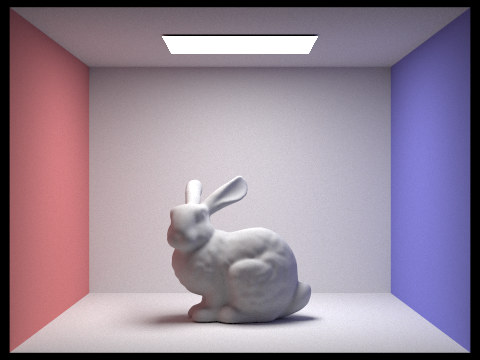
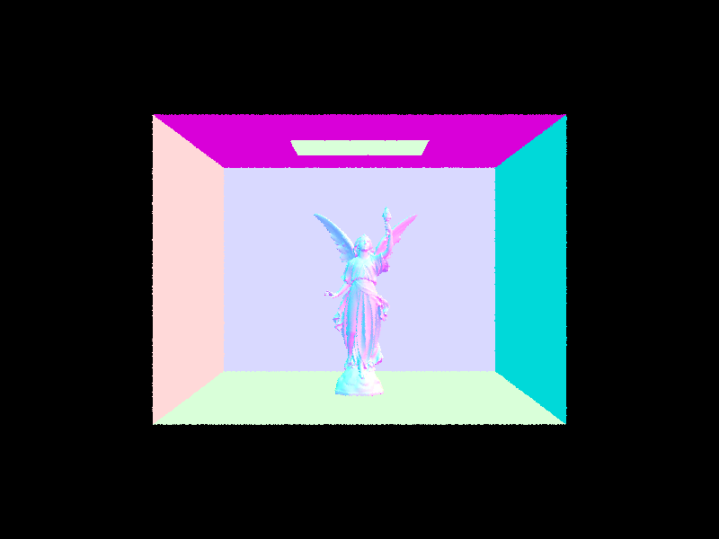
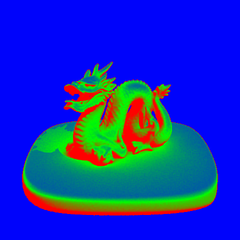
Normal Shading Example

Part 2: Bounding Volume Hierarchy

To construct a Hierarchical Space Partitioning to accelerate ray-scene intersection, Bounding Volume Hierarchy tree is usually used in ray tracing. Like any other binary tree, BVH is constructed by recursively splitting the primitives into two subsets until the number of primitives in a leaf node is less than given maxLeafSize threshold.

The engineering idea of BVH is quite clear:

1. Compute the bounding box of all primitives in the current range.

2. If the range is small enough, create a leaf node that stores [start, end) directly.

3. Otherwise, compute the centroid bounding box and choose the split axis as its maximum-extent dimension.

4. Try to partition the primitives into two subsets based on the selected axis. Here we can simply use the median of the centroids along the split axis as the splitting plane, and partition the primitives into two subsets based on whether their centroids are less than or greater than the splitting plane.

5. Recursively build the left subtree from [start, mid) and the right subtree from [mid, end).

After building the BVH tree, we then perform intersection tests by traversing the tree. The process can be described as follows:

function intersectBVH(ray, node) {
    if (node is a leaf) {
        // Test intersection with all primitives in the leaf
        for each primitive in node.primitives {
            test ray-primitive intersection and update closest hit
        }
    } else {
        // Test intersection with the bounding boxes of the child nodes
        if (ray intersects node.left.boundingBox) {
            intersectBVH(ray, node.left);
        }
        if (ray intersects node.right.boundingBox) {
            intersectBVH(ray, node.right);
        }
        compare the hits from left and right child and keep the closest one
    }
}

Noting that the bool BBox::intersect(const Ray& r, double& t0, double& t1) function will change t0 and t1 somehow, which requires attention to variable passed and updated in the recursive calls.

Heuristic Partition

The median split heuristic is trivial and easy to come up with. However, when we inspect some bad cases like the one shown below, we can see that the median split can lead to very unbalanced trees and poor performance.

Comparison across BVH and No BVH

We select a moderately complex scene with 10k+ primitives to fully test the advantages of BVH.
The scene is rendered with the same settings (800 x 600 resolution)
The rendering time is displayed in the following table, the BVH implementation achieves a significant speedup of around 1640x compared to the naive approach without BVH, which demonstrates the effectiveness of hierarchical space partitioning in accelerating ray-scene intersection tests.

Method (5 runs)	Average Time (s)	Relative Speedup
No BVH	139.1515	1.0x
BVH	0.08484	1640x

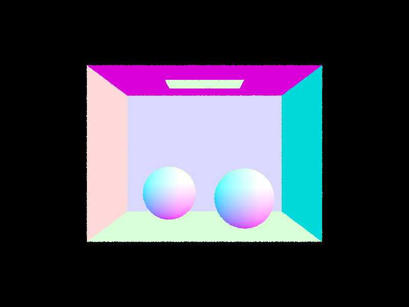
Test Scene

Part 3: Direct Illumination

Hemisphere Sampling

This method uses a more straightforward idea: instead of sampling the lights directly, it randomly samples directions over the hemisphere above the hit point and checks whether those rays happen to reach a light source. If a sampled ray hits an emissive object, its contribution is added using the BSDF, the cosine term, and the sampling PDF. After many samples, the results are averaged to estimate the direct lighting.

This approach is simple, but it is not very efficient. Since most random directions do not hit a light, many samples contribute nothing, which makes the image noisier.

Light Importance Sampling

This method is more focused because it samples the lights themselves instead of random directions. For each light, it generates one or more sample directions toward that light, then casts a shadow ray to check whether the light is actually visible from the hit point. If the light is not blocked, its contribution is added to the final result.

Because the samples are taken from actual light sources, this method wastes fewer samples and usually converges much faster. In practice, it produces cleaner lighting and less noise than hemisphere sampling.

Scene Comparison

We use the following commands to render the same scene with hemisphere sampling and light importance sampling, and compare the results.

# Render with hemisphere sampling
./pathtracer -t 8 -s 64 -l 32 -m 6 -H -f CBspheres_64_32_h.png -r 480 480 ../dae/sky/CBspheres_lambertian.dae
# Render with light importance sampling
./pathtracer -t 8 -s 64 -l 32 -m 6 -f CBspheres_64_32_l.png -r 480 480 ../dae/sky/CBspheres_lambertian.dae

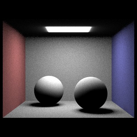
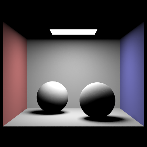
On the left is the result from hemisphere sampling, which is quite noisy and dimmed in the side areas. On the right is the result from light importance sampling, which is much cleaner and brighter, especially around the light sources. This clearly demonstrates the advantage of importance sampling for direct lighting.

Light Ray Count

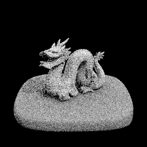
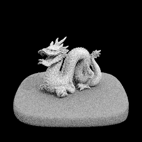
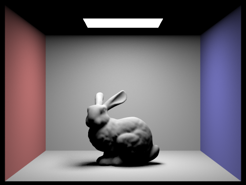
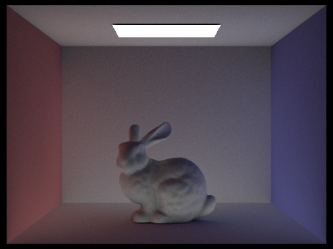
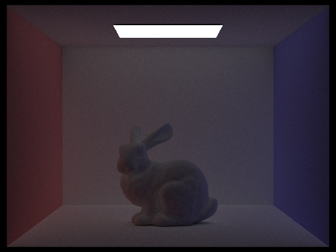
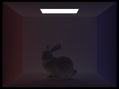
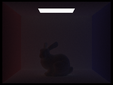
We focus on rendering the /dae/sky/dragon.dae scene and compare the noise levels in soft shadows when rendering with 1, 4, 16, and 64 light rays (the -l flag) and with 1 sample per pixel (the -s flag) using light sampling. The results are shown below:

1 Light Ray	4 Light Rays
16 Light Rays	64 Light Rays

As the number of light rays increases, the noise and graininess in the soft shadow areas significantly decrease, resulting in smoother and more realistic shadows. With only 1 light ray, the shadows are very noisy and patchy. With 4 light rays, the noise is reduced but still noticeable. With 16 light rays, the shadows become much smoother, and with 64 light rays, the shadows are very clean and well-defined. This clearly illustrates how increasing the number of light rays can improve the quality of direct lighting in ray tracing.

Conclusion

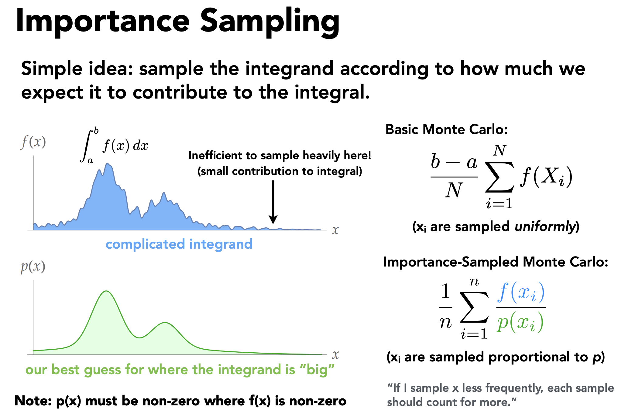
This slides emphasizes that light importance sampling is more prioritized as the curve of the integral is much smoother and more focused around the peaks, while hemisphere sampling is more noisy and has a lot of variance.
In short, hemisphere sampling chooses random directions first and hopes they hit a light, while importance sampling chooses the light first and then checks visibility. That is why importance sampling is generally more accurate and efficient for direct lighting.

Part 4: Global Illumination

My indirect lighting is implemented in at_least_one_bounce_radiance.The idea is to recursively trace one randomly sampled bounce at a time and accumulate the light that comes back from deeper paths.

The function first keeps the direct-lighting term by calling one_bounce_radiance when direct illumination should be included in the result. If the ray has no remaining depth, it simply returns that value.

For indirect lighting, it samples a new direction from the BSDF at the current surface. This gives the incoming direction, the BSDF value, and the sampling PDF. If the sample is invalid or goes below the surface, the path ends there.

To avoid tracing unnecessarily long paths, I use Russian roulette with a continuation probability of 0.65. If the path survives, I transform the sampled direction back to world space, spawn the next ray, and intersect it with the scene. If the new ray hits nothing, there is no additional indirect contribution. If it does hit something, I recursively evaluate the radiance at that next intersection.

Finally, I add the indirect term using the usual Monte Carlo weighting: multiply the returned radiance by the BSDF and cosine term, then divide by the PDF and the Russian roulette continuation probability. So the final result is the direct contribution at the current point plus the recursively estimated bounced light.

Pseudocode

function at_least_one_bounce_radiance(ray, depth) {
    L = direct lighting at current hit

    if depth limit reached:
        return L

    sample wi from BSDF
    if sample invalid:
        return L

    with probability cp:
        trace next ray along wi
        if next ray hits:
            L_next = indirect lighting at next hit
            L += f * L_next * cos(theta) / (pdf * cp)

    return L
}

Difference between Levels of Max Bounce Depths

m = 0	m = 1	m = 2	m = 3	m = 4	m = 5

Part 5: Adaptive Sampling

Adaptive sampling adopts a more intelligent approach to sampling by allocating more samples to pixels that are likely to have higher variance (e.g., edges, shadows) and fewer samples to smoother areas. This can significantly reduce noise while keeping the rendering time manageable.

To reproduce the pipeline of adaptive sampling, we can follow these steps:

1. Like former procedures, we first render the image with a given batch size samplesPerBatch and accumulate the results for each pixel.
2. After each batch, we compute the variance of the accumulated samples for each pixel. This can be done using the formula:

$$\begin{aligned} S_1 &= \sum_{i=1}^{n} x_i \\ S_2 &= \sum_{i=1}^{n} x_i^2 \\ \sigma^2 &= \frac{S_2 - \frac{S_1^2}{n}}{n - 1} \end{aligned}$$

3. We then compute the tolerance condition $I < \text{MaxTolerance} \times \mu$, where $I$ is the z-value of current batch, $\mu$ is the mean of the accumulated samples.
4. Once the condition is satisfied, we stop sampling for that pixel and move on to the next one. Otherwise, we continue sampling until we reach the maximum number of samples maxSamples or the tolerance condition is met.
5. Update the sample buffer with the final accumulated color for each pixel and fulfill the number of samples used for that pixel.

The examples and sample rate heatmap of the rendered images with adaptive sampling are shown below:

As we can see, after applying adaptive sampling, the sample rate is much higher around the edges and shadow areas, which are more likely to have higher variance. Whereas in the smoother areas, the sample rate is significantly reduced, which helps to save rendering time while still maintaining good image quality. The final rendered image with adaptive sampling is much cleaner and less noisy compared to uniform sampling, especially in the shadow regions and around the edges of objects.

(Optional) Part 6: Extra Credit Opportunities

Surface Area Heuristic (SAH) for BVH Construction

To go beyond the centroid midpoint split used in Part 2, I studied the Surface Area Heuristic (SAH) formulation from PBRT 3rd Edition, Section 4.3.2. The core idea is to stop treating BVH construction as a purely geometric partitioning problem and instead choose the split that minimizes the expected ray traversal cost.

The weakness of a naive midpoint split is that it only looks at centroid positions. It does not reason about how large the two child bounding boxes will become, how much they overlap, or how many primitives will likely be tested after the split. As illustrated in the PBRT figure below, a midpoint cut can easily produce two children with large overlapping bounds, which leads to unnecessary traversal work.

Source: PBRT 3e, Figure 4.4.

If a node contains $N$ primitives and we decide to keep it as a leaf, the expected cost is

$$C_{\text{leaf}} = N \, C_{\text{isect}},$$

where $C_{\text{isect}}$ is the cost of one ray-primitive intersection test.

If we instead split the node into two children $L$ and $R$, SAH estimates the cost as

$$C_{\text{split}} = C_{\text{trav}} + P(L \mid P)\, N_L \, C_{\text{isect}} + P(R \mid P)\, N_R \, C_{\text{isect}},$$

where $C_{\text{trav}}$ is the cost of traversing an interior node, $P(L \mid P)$ and $P(R \mid P)$ are the conditional probabilities that a ray passing through the parent node $P$ also intersects the left or right child, and $N_L, N_R$ are the primitive counts in the two children.

Using geometric probability, PBRT approximates these probabilities by surface-area ratios:

$$P(L \mid P) = \frac{S_L}{S_P}, \qquad P(R \mid P) = \frac{S_R}{S_P},$$

so the split cost becomes

$$C_{\text{split}} = C_{\text{trav}} + \frac{S_L}{S_P} N_L C_{\text{isect}} + \frac{S_R}{S_P} N_R C_{\text{isect}}.$$

Following PBRT’s normalization $C_{\text{isect}} = 1$ and $C_{\text{trav}} = 1/8$, this simplifies to

$$C_{\text{split}} = 0.125 + \frac{N_L S_L + N_R S_R}{S_P}.$$

This equation explains why SAH is stronger than midpoint splitting:

1. It penalizes large child bounds through $S_L$ and $S_R$.
2. It penalizes badly unbalanced primitive distributions through $N_L$ and $N_R$.
3. It naturally decides not to split when the leaf cost is already cheaper.

PBRT-Style Bucketed SAH Walk-Through

PBRT does not evaluate every possible partition exactly. Instead, it uses a practical approximation:

1. Compute the bounding box of the current node and the bounding box of primitive centroids.
2. Choose the split axis as the maximum-extent axis of the centroid bounds.
3. Project centroids onto that axis and place them into 12 buckets.
4. For each bucket boundary, compute the union bounds and primitive counts on the left and right sides.
5. Evaluate the SAH cost at each boundary and choose the minimum.
6. Compare that minimum cost against the leaf cost; split only when the split is worth it.

Source: PBRT 3e, Figure 4.6.

To make the process concrete, I reproduced a small 8-primitive node and evaluated the root split exactly with the bucketed SAH formula above. The centroid range on the chosen axis is $[0.0862, 0.8737]$, so the naive midpoint plane would be at $x = 0.4799$.

The occupied buckets are:

Occupied Bucket	Centroid Range on Split Axis	Primitive Count
B0	$[0.0862, 0.1518)$	3
B3	$[0.2831, 0.3487)$	1
B4	$[0.3487, 0.4143)$	1
B5	$[0.4143, 0.4799)$	1
B10	$[0.7424, 0.8080)$	1
B11	$[0.8080, 0.8737]$	1

Evaluating the candidate boundaries gives:

Candidate	Meaning	Estimated Cost
Split after B4	Minimum-cost split chosen by SAH	1.9911
Split after B5	Naive centroid midpoint split	4.7654
No split	Leaf cost with 8 primitives	8.0000

In this node alone, the SAH-selected split reduces the expected cost by

$$\frac{4.7654 - 1.9911}{4.7654} \approx 58.2\%$$

relative to the naive midpoint split. This is exactly the kind of case where midpoint partitioning looks “reasonable” geometrically, but still produces a much worse traversal cost because the two children inherit large and overlapping bounds.

Standalone Micro-Benchmark

Since this blog repository only contains the write-up rather than the full CS184 ray tracer, I validated the idea with a standalone AABB-only BVH benchmark that mirrors PBRT’s assumptions:

1. maxLeafSize = 4
2. midpoint BVH versus 12-bucket SAH BVH
3. 4,000 random rays shot from outside the scene bounds
4. weighted traversal cost reported as $0.125 \cdot N_{\text{node}} + N_{\text{prim}}$, matching PBRT’s $C_{\text{trav}} / C_{\text{isect}} = 1/8$

The first scene uses 800 uniformly distributed random boxes, while the second scene repeats the hard 8-primitive pattern above 100 times to stress-test midpoint splitting.

Scene	Method	Build Time (s)	Avg. Nodes Visited	Avg. Primitive Tests	Avg. Weighted Cost
Uniform random boxes (800)	Midpoint	0.0062	43.754	14.732	20.201
Uniform random boxes (800)	SAH	0.0242	38.559	12.615	17.435
Repeated hard pattern (800)	Midpoint	0.0116	12.298	1.617	3.154
Repeated hard pattern (800)	SAH	0.0162	9.615	1.299	2.501

The relative improvements are:

Scene	Node Visits Reduction	Primitive-Test Reduction	Weighted-Cost Reduction	Build-Time Multiplier
Uniform random boxes	11.9%	14.4%	13.7%	3.9x
Repeated hard pattern	21.8%	19.7%	20.7%	1.4x

These results match the expected SAH trade-off very well: it spends more time during construction, but it consistently builds a BVH that is cheaper to traverse. In other words, midpoint splitting is cheaper now, while SAH is cheaper every time a ray is traced later. For a ray tracer, especially on scenes with thousands of primitives and many camera/shadow rays, that is almost always the better trade.

Overall, SAH is a much better fit for BVH construction because it optimizes the quantity that actually matters at render time: expected traversal work. The midpoint heuristic is still attractive as a baseline because it is simple and fast, but once the scene distribution becomes skewed or overlap-heavy, SAH provides a far more reliable cost model and produces meaningfully better trees.